Graph Learning.

Learn the graph from EEG signals using the algorithm proposed by Kalofolias et al. (2019) and implemented in pygsp2. This example follows the methods described in Miri et al. (2024). To run this example download the following data file data_set_IVa_aa.mat from the BCI Competition III:

https://www.bbci.de/competition/download/competition_iii/berlin/100Hz/data_set_IVa_aa_mat.zip

You need to decompress the file and place the file in a directory named data.

import os

import sys
from pathlib import Path

import matplotlib.pyplot as plt
import mne
import numpy as np
from scipy.io import loadmat

from eegrasp import EEGrasp
from eegrasp.utils_examples import fetch_data

# Instantiate EEGraSP
gsp = EEGrasp()

current_dir = os.getcwd()
os.chdir(os.path.dirname(current_dir))
assets_dir = Path('..') / Path('data')
fetch_data(assets_dir, database='graph_learning')
file_name = os.path.join(assets_dir, '100Hz', 'data_set_IVa_aa.mat')

try:
    data = loadmat(file_name)
except (FileNotFoundError, OSError):
    print(f'File {file_name} not found')
    sys.exit(-1)

eeg = (data['cnt']).astype(float) * 1e-7  # Recommendation: to set to V
events = np.squeeze(data['mrk'][0, 0][0])
info = data['nfo'][0, 0]
ch_names = [ch_name[0] for ch_name in info[2][0, :]]
FS = info[1][0, 0]
pos = np.array([info[3][:, 0], info[4][:, 0]]).T

Downloading data file to:
 ../data/data_set_IVa_aa.mat

# Create structure
mne_info = mne.create_info(ch_names=ch_names, sfreq=FS, ch_types='eeg')
data = mne.io.RawArray(eeg.T, mne_info)

# Extract events and annotate
mne_events = np.zeros((len(events), 3))
mne_events[:, 0] = events
annotations = mne.annotations_from_events(mne_events, FS)
data = data.set_annotations(annotations)
events2, events_id = mne.events_from_annotations(data)

# Reference data to average
data, _ = mne.set_eeg_reference(data, ref_channels='average')

# Filter between 8 and 30 Hz
data = data.filter(l_freq=8, h_freq=30, n_jobs=-1)

# Epoch and Crop epochs
epochs = mne.Epochs(data, events2, tmin=0.0, tmax=2.5, baseline=(0, 0.5), preload=True)
epochs = epochs.crop(0.5, None)

epochs_data = epochs.get_data(copy=False)

Creating RawArray with float64 data, n_channels=118, n_times=298458
    Range : 0 ... 298457 =      0.000 ...  2984.570 secs
Ready.
Used Annotations descriptions: [np.str_('0.0')]
EEG channel type selected for re-referencing
Applying average reference.
Applying a custom ('EEG',) reference.
Filtering raw data in 1 contiguous segment
Setting up band-pass filter from 8 - 30 Hz

FIR filter parameters
---------------------
Designing a one-pass, zero-phase, non-causal bandpass filter:
- Windowed time-domain design (firwin) method
- Hamming window with 0.0194 passband ripple and 53 dB stopband attenuation
- Lower passband edge: 8.00
- Lower transition bandwidth: 2.00 Hz (-6 dB cutoff frequency: 7.00 Hz)
- Upper passband edge: 30.00 Hz
- Upper transition bandwidth: 7.50 Hz (-6 dB cutoff frequency: 33.75 Hz)
- Filter length: 165 samples (1.650 s)

[Parallel(n_jobs=-1)]: Using backend LokyBackend with 2 concurrent workers.
[Parallel(n_jobs=-1)]: Done  38 tasks      | elapsed:    1.1s
[Parallel(n_jobs=-1)]: Done 118 out of 118 | elapsed:    2.0s finished
Not setting metadata
280 matching events found
Applying baseline correction (mode: mean)
0 projection items activated
Using data from preloaded Raw for 280 events and 251 original time points ...
0 bad epochs dropped

gsp.data = epochs_data
gsp.coordinates = pos
W, Z = gsp.learn_graph(a=0.34, b=0.4)

gsp.compute_graph(W)

tril_idx = np.tril_indices(len(Z), -1)

  0%|          | 0/280 [00:00<?, ?it/s]
  8%|▊         | 23/280 [00:00<00:01, 220.45it/s]
 16%|█▋        | 46/280 [00:00<00:01, 221.31it/s]
 25%|██▍       | 69/280 [00:00<00:00, 221.59it/s]
 33%|███▎      | 92/280 [00:00<00:00, 221.77it/s]
 41%|████      | 115/280 [00:00<00:00, 221.83it/s]
 49%|████▉     | 138/280 [00:00<00:00, 221.76it/s]
 57%|█████▊    | 161/280 [00:00<00:00, 221.80it/s]
 66%|██████▌   | 184/280 [00:00<00:00, 221.78it/s]
 74%|███████▍  | 207/280 [00:00<00:00, 221.78it/s]
 82%|████████▏ | 230/280 [00:01<00:00, 221.79it/s]
 90%|█████████ | 253/280 [00:01<00:00, 221.79it/s]
 99%|█████████▊| 276/280 [00:01<00:00, 221.77it/s]
100%|██████████| 280/280 [00:01<00:00, 221.66it/s]
Found solution after 241 iterations

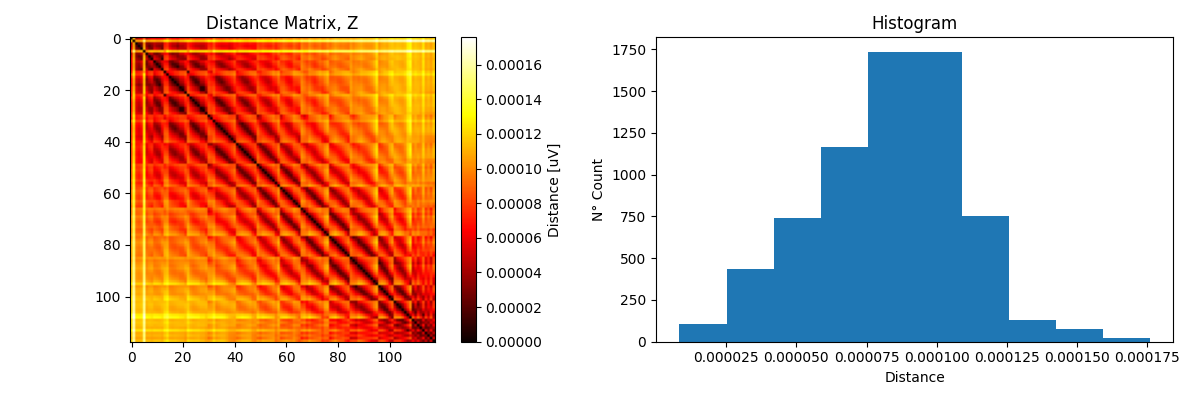
plt.figure(figsize=(12, 4))
plt.subplot(121)
plt.imshow(Z, cmap='hot')
plt.colorbar(label='Distance [uV]')
plt.title('Distance Matrix, Z')

plt.subplot(122)
plt.hist(Z[tril_idx], 10)
plt.xlabel('Distance')
plt.ylabel('N° Count')
plt.title('Histogram')
plt.tight_layout()

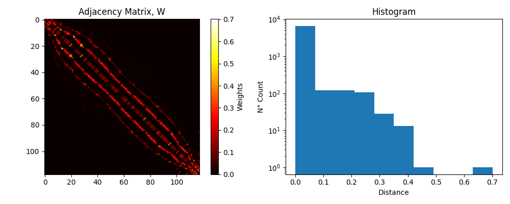
plt.figure(figsize=(10, 4))
plt.subplot(121)
plt.imshow(W, cmap='hot')
plt.colorbar(label='Weights')
plt.title('Adjacency Matrix, W')

plt.subplot(122)
plt.hist(W[tril_idx], bins=10, log=True)
plt.xlabel('Distance')
plt.ylabel('N° Count')
plt.title('Histogram')

plt.tight_layout()

G = gsp.graph
G.set_coordinates(pos)
G.compute_laplacian()
G.compute_fourier_basis()
eigenvectors = np.array(G.U)
eigenvalues = np.array(G.e)

size = np.sum(G.W.toarray(), axis=0) / max(np.sum(G.W.toarray(), axis=0))
weights = G.W.toarray()
tril_idx = np.tril_indices(len(weights), -1)

wh = []
for i in range(len(tril_idx[0])):
    x, y = tril_idx[0][i], tril_idx[1][i]
    if weights[x, y] != 0:
        wh.append(weights[x, y])

G.plot(vertex_color=eigenvectors[:, 5], vertex_size=size, cmap='magma', alphan=0.9,
       alphav=0.5, edge_weights=wh)

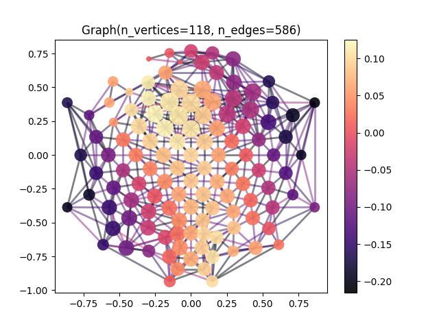
(<Figure size 640x480 with 2 Axes>, <Axes: title={'center': 'Graph(n_vertices=118, n_edges=586)'}>)

plt.figure()
plt.scatter(eigenvalues, np.arange(0, len(eigenvalues)), s=50, color='purple')
plt.plot(eigenvalues, np.arange(0, len(eigenvalues)), linewidth=3, color='black')
plt.xlabel('Eigenvalue')
plt.ylabel('Eigenvalue Index')

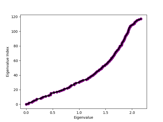
Text(38.347222222222214, 0.5, 'Eigenvalue Index')

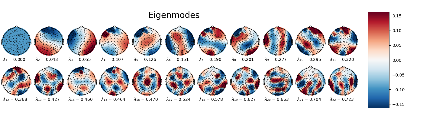
SCALE = 0.2
vlim = (-np.amax(np.abs(eigenvectors)) * SCALE, np.amax(np.abs(eigenvectors)) * SCALE)

fig, axs = plt.subplots(2, 11, figsize=(14, 4))
for i, ax in enumerate(axs.flatten()):
    im, cn = mne.viz.plot_topomap(eigenvectors[:, i], pos, sensors=True, axes=ax,
                                  cmap='RdBu_r', vlim=vlim, show=False, sphere=0.9)
    CORE = r'\u208'
    SUBSCRIPT = [(CORE + i + '').encode().decode('unicode_escape') for i in str(i + 1)]
    SUBSCRIPT = ''.join(SUBSCRIPT)
    ax.text(-0.9, -1.3, r'$\lambda$' + SUBSCRIPT + ' = ' + f'{eigenvalues[i]:.3f}')

fig.subplots_adjust(0, 0, 0.85, 1, 0, -0.5)
cbar = fig.add_axes([0.87, 0.1, 0.05, 0.8])
plt.colorbar(im, cax=cbar)
fig.text(0.35, 0.85, 'Eigenmodes', size=20)
plt.show()

Estimated memory usage: 977 MB